by Matteo Picchiani, PhD GMATICS
GMATICS has implemented examples of land cover classification through the DYDAS platform, that were also shown at AIT 2021 and IGARSS 2022 conferences.
The DYDAS infrastructure has been tested, in fact, with Copernicus Sentinel-1 (S1) and Sentinel-2 (S2) data for implementing a ML supervised classification task. The satellite data have been collected over the province of Milan (Italy) by considering the acquisition on 08 April, 2015 and 17 April, 2020 for S1 and 08 June, 2015 and 11 April, 2020, for S2 products respectively.
The Sentinel-1 satellites carry an advanced synthetic aperture radar (SAR) instrument to provide all-weather, day-and-night imagery of Earth’s surface. The C-band SAR instrument can have a spatial resolution down to 5 m and a swath width up to 400 km. The orbit has a 12-day repeat cycle and two satellites give a 6 day revisit time.
The C-band data is used for change detection, sea ice monitoring, ocean maritime navigation and vegetation mapping.
In the test case a Level-2 GRD data has been considered. The dataset has been assimilated on the DYDAS Data Lake, using the GDA functionalities and the HH and HV polarizations images have been converted into 𝜎𝑜.
The Sentinel-2 Multiple Spectral Imager (MSI) records 13 spectral bands across the visible and infrared portions of the electromagnetic spectrum at different spatial resolutions from 10 m to 60 m depending on their operation and use. There are currently two Sentinel-2 satellites in suitably phased orbits to give a revisit period of 5 days at the Equator and 2-3 days at European latitudes. Being an optical sensor they are of course also affected by cloud cover and illumination conditions. The two satellites have been fully operational since 2017 and record continuously over land and the adjacent coastal sea areas. Their specification represents a continuation and upgrade of the US Landsat system which has archive data stretching back to the mid 1980s. In this test a L2 S2 product has been assimilated on the DYDAS Data Lake by exploiting the GDA functions.
The S1 and S2 data have been co-registrated and staked directly on the processing on the HPC infrastructure. Two staks have been produced for 2015 and 2020 respectively. Finally, to test further the GDA functionalities, a shapefile of the Milan province boundaries has been used to mask the pixels outside the province border on the two datasets.
A supervised Neural Network model has been trained using the DYDAS HPC. A shallow NN architecture has been adopted with the following topology: 11 – 10 – 5 – 4.
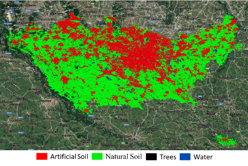
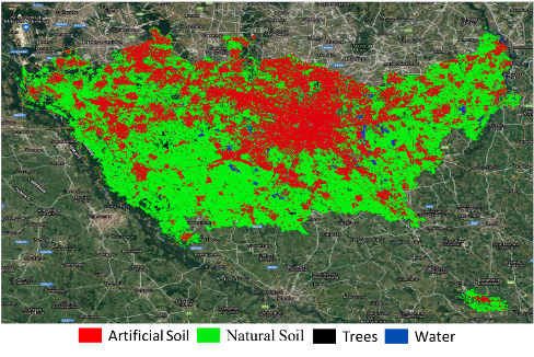
The first layer of the topology is composed by 11 neurons to accepts the selected bands of the S1 – S2 stack. Were considered the two polarization of the S1 data and the following bands (with 10 m and 20 m of spatial resolution) of S2: B2, B3, B4, B5, B6, B7, B8, B11 and B12. Looking at the following layers of the NN topology, two hidden layers of 10 and 5 neurons have been respectively considered, while the last layer provides the four outputs considered for the classification. We considered here four macro classes as: Natural Soil (including crops, grassland and baresoil), Trees, Water and Artificial Soil.
As training information the CORINE Land Cover of 2018 has been considered. This latter is available in tiled GeoTiff format and the tiles over the AoI have been assimilated and treated on the DYDAS platform as done for the Satellite data.

The NN has been trained with the stack of the S1-S2 products of 2015 and then applied to the 2020 data.
The training set pre-processing has been carried out by a dedicated python script to build the input-output patterns directly on the DYDAS platform. This pre-processing operation runs in few seconds. Then the NN has been trained by using a python – Tensorflow model directly on the HPC infrastructure. We tested several runs of the model training phase. We recorded a very good performance with respect the training time, since the 1000 epochs needed to the model convergence have been executed always in less than 3 minutes.
The NN output has been finally compared with the CORINE reference map, registering an overall accuracy of 98% and K-coefficient equal to about 0.89. These good performance is also confirmed by the visual comparison of the NN output and the CORINE reference map.

Classificazione delle immagini satellitari: l’attuazione del modello ML
a cura di Matteo Picchiani, PhD GMATICS
GMATICS ha implementato esempi di classificazione della copertura del suolo attraverso la piattaforma DYDAS, che sono stati mostrati anche alle conferenze AIT 2021 e IGARSS 2022.
L’infrastruttura DYDAS è stata testata, infatti, con i dati di Copernicus Sentinel-1 (S1) e Sentinel-2 (S2) per l’implementazione di un compito di classificazione supervisionato ML. I dati satellitari sono stati raccolti sulla provincia di Milano (Italia) considerando l’acquisizione l’8 aprile 2015 e il 17 aprile 2020 rispettivamente per S1 e 08 giugno 2015 e 11 aprile 2020 per i prodotti S2.
I satelliti Sentinel-1 trasportano uno strumento radar ad apertura sintetica (SAR) avanzato per fornire immagini per tutte le stagioni, giorno e notte della superficie terrestre. Lo strumento SAR in banda C può avere una risoluzione spaziale fino a 5 m e una larghezza di fascia fino a 400 km. L’orbita ha un ciclo di ripetizione di 12 giorni e due satelliti danno un tempo di rivisitazione di 6 giorni.
I dati in banda C vengono utilizzati per il rilevamento delle modifiche, il monitoraggio del ghiaccio marino, la navigazione marittima oceanica e la mappatura della vegetazione.
Nel caso di prova sono stati presi in considerazione dati GRD di livello 2. Il set di dati è stato assimilato sul DYDAS Data Lake, utilizzando le funzionalità GDA e le immagini di polarizzazione HH e HV sono state convertite in σo.
Il Sentinel-2 Multiple Spectral Imager (MSI) registra 13 bande spettrali attraverso le porzioni visibili e infrarosse dello spettro elettromagnetico a diverse risoluzioni spaziali da 10 m a 60 m a seconda del loro funzionamento e utilizzo. Attualmente ci sono due satelliti Sentinel-2 in orbite opportunamente graduali per dare un periodo di rivisitazione di 5 giorni all’equatore e 2-3 giorni alle latitudini europee. Essendo un sensore ottico, sono ovviamente influenzati anche dalla copertura nuvolosa e dalle condizioni di illuminazione. I due satelliti sono pienamente operativi dal 2017 e registrano continuamente sulla terraferma e sulle aree marittime costiere adiacenti. La loro specifica rappresenta una continuazione e un aggiornamento del sistema Landsat degli Stati Uniti che ha dati di archivio che risalgono alla metà degli anni 1980. In questo test un prodotto L2 S2 è stato assimilato sul DYDAS Data Lake sfruttando le funzioni GDA.
I dati S1 e S2 sono stati co-registrati e puntati direttamente sull’elaborazione sull’infrastruttura HPC. Due doghe sono state prodotte rispettivamente per il 2015 e il 2020. Infine, per testare ulteriormente le funzionalità GDA, è stato utilizzato uno shapefile dei confini della provincia di Milano per mascherare i pixel al di fuori del confine provinciale sui due dataset.
Un modello di rete neurale supervisionato è stato addestrato utilizzando l’HPC DYDAS. È stata adottata un’architettura NN poco profonda con la seguente topologia: 11 – 10 – 5 – 4.
Il primo strato della topologia è composto da 11 neuroni per accettare le bande selezionate dello stack S1 – S2. Consideriamo le due polarizzazioni dei dati S1 e le seguenti bande (con 10 m e 20 m di risoluzione spaziale) di S2: B2, B3, B4, B5, B6, B7, B8, B11 e B12. Osservando i seguenti livelli della topologia NN, sono stati considerati rispettivamente due strati nascosti di 10 e 5 neuroni, mentre l’ultimo livello fornisce i quattro output considerati per la classificazione. Abbiamo considerato qui quattro macro classi come: Suolo naturale (comprese colture, prati e terra nuda), Alberi, Acqua e Suolo artificiale.
Come informazione sulla formazione è stata presa in considerazione la copertura del suolo CORINE del 2018. Quest’ultimo è disponibile in formato GeoTiff piastrellato e le tessere sopra l’AoI sono state assimilate e trattate sulla piattaforma DYDAS come fatto per i dati satellitari.
L’NN è stato addestrato con lo stack dei prodotti S1-S2 del 2015 e quindi applicato ai dati del 2020.
La pre-elaborazione del set di formazione è stata effettuata da uno script python dedicato per costruire i modelli di input-output direttamente sulla piattaforma DYDAS. Questa operazione di pre-elaborazione viene eseguita in pochi secondi. Quindi l’NN è stato addestrato utilizzando un modello python – Tensorflow direttamente sull’infrastruttura HPC. Sono state testate diverse esecuzioni della fase di training del modello. Abbiamo registrato un’ottima performance rispetto al tempo di allenamento, dal momento che le 1000 epoche necessarie alla convergenza del modello sono state eseguite sempre in meno di 3 minuti.
L’output NN è stato infine confrontato con la mappa di riferimento CORINE, registrando una precisione complessiva del 98% e un coefficiente K pari a circa 0,89. Queste buone prestazioni sono confermate anche dal confronto visivo dell’uscita NN e della mappa di riferimento CORINE.